XGBoost （三）计算案例-XGBoost（Extreme Gradient Boosting，极端梯度提升树）-老孟讲编程

样本 i	x	y
1	1	2.1
2	2	4.0
3	3	6.2
4	4	8.1
5	5	10.0
6	6	12.2
7	7	14.1
8	8	16.0
9	9	18.1
10	10	20.2

损失函数：平方损失，λ = 1, γ = 0

损失函数一阶导和二阶导计算公式：

初始预测取均值：

计算每个样本的一阶导和二阶导值：

样本 i	x	y	基础预测	一阶导	二阶导
1	1	2.1	11.1	9.0	1
2	2	4.0	11.1	7.1	1
3	3	6.2	11.1	4.9	1
4	4	8.1	11.1	3.0	1
5	5	10.0	11.1	1.1	1
6	6	12.2	11.1	-1.1	1
7	7	14.1	11.1	-3.0	1
8	8	16.0	11.1	-4.9	1
9	9	18.1	11.1	-7.0	1
10	10	20.2	11.1	-9.1	1

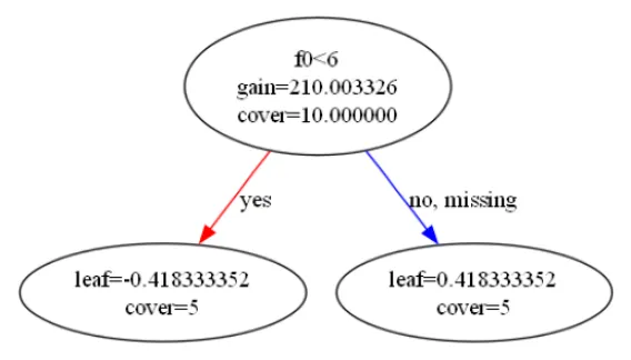
我们以分裂点 x < 6 为例，计算下其分裂增益：

节点	样本集合	一阶导和 (G)	二阶导和 (H)
左子集	(1, 2, 3, 4, 5)	25.1	5
右子集	(6, 7, 8, 9, 10)	-25.1	5
父节点	所有样本	0	10

带入到分裂增益计算公式中：

Gain = 0.5 ∗ (105.0 + 105.0 − 0)−0 = 0.5 ∗ 210.0 = 105.0

最后计算下叶子节点的输出值：

# pip install scikit-learn
# pip install xgboost
# pip install matplotlib

from xgboost import XGBRegressor, plot_tree
import numpy as np
import matplotlib.pyplot as plt

def demo():
    # 构造数据
    x = np.array([1,2,3,4,5,6,7,8,9,10]).reshape(-1,1)
    y = np.array([2.1,4.0,6.2,8.1,10.0,12.2,14.1,16.0,18.1,20.2])

    # 训练模型
    xgb = XGBRegressor(n_estimators=2, max_depth=2, learning_rate=0.1, objective='reg:squarederror')
    xgb.fit(x, y)

    # 绘制每棵树
    for idx in range(xgb.n_estimators):
        plt.figure(figsize=(12,8), dpi=150)  # 调整图像大小和分辨率
        plot_tree(xgb, tree_idx=idx, rankdir='LR', with_stats=True)  # 'LR' 横向展示
        plt.show()

    xgb.predict

if __name__ == '__main__':
    demo()