感知机（Perceptron）是1958 年由弗兰克·罗森布拉特（Frank Rosenblatt）提出的一个经典线性分类算法。它是机器学习领域最早提出的基于数学规则进行分类的模型之一，适用于解决二分类问题。

作为一种线性分类算法，感知机能够快速处理线性可分的二分类问题，且实现起来非常容易。然而，它只能解决线性可分的问题，对于非线性可分的数据无法有效分类。感知机对噪声非常敏感，错误的标签或异常数据会导致模型的不稳定。

简言之：感知机算法适合线性可分的问题场景。

1. 基本原理

接下来，我们将探讨感知机算法如何进行分类，以及训练。

1.1 预测过程

感知机是一个线性分类器，公式表示如下：

\( w \) 表示权重向量, \( b \) 表示偏置, \( x \) 表示输入向量, \( sign(·) \) 表示符号函数。

当预测某个数据的类别，感知机会根据输入数据的特征计算得到决策函数值，然后根据该决策函数值的符号来决定其类别。如果为 > 0，归类为 +1 类别，如果 <= 0，则归类到 -1 类别。

注意：感知机算法在内部使用 +1 和 -1 来表示两个类别，这个不同于某些二分类算法使用 0 和 1 来表示两个类别。

对于权重向量 \( w \) 和偏置 \( b \) 的理解：

权重向量 \( w \) 表示每个特征对预测结果的影响程度，特征权重越大，表示该特征越能影响分类预测的结果。特征的权重可以是正的也可以是负的，表明某个特征对分类预测贡献是 推动分类结果为正 还是 推动分类结果为负。

偏置项 b 的作用是调整决策边界的位置。如果没有偏置项，感知机的决策边界总是会经过原点，这会限制模型的拟合能力，使它无法适应某些分布的数据。如果数据已经进行了标准化（Standardization）或归一化（Normalization），特别是特征均值被调整为 0，那么偏置的作用可能会被抵消。这种情况下，偏置可以被省略而不影响模型性能。

最后需要明确，对于感知机，权重向量 \( w \) 和偏置 \( b \) 是算法要学习的参数。

1.2 训练过程

感知机训练的目标是不断调整参数 \( w \) 和 \( b \) ，使得训练数据中尽可能多的样本能够被分类正确，感知机的学习效果就越好。感知机通过使用：误分类样本的损失函数 来表示模型对训练数据的学习效果。对于一个给定的样本 \( (x_i, y_i) \)，其损失定义为：

正确分类：当 \( y_{i}(w^{T}x + b) > 0 \) 时，预测正确，损失为 0。
错误分类：当 \( y_{i}(w^{T}x + b) \leq 0 \) 时，预测错误，损失为 \(−y_{i}(w^{T}x + b)\)，即对错误分类样本的惩罚。

将所有样本的损失值累加一起，就表示感知机的训练效果。损失值越小，训练效果越好，损失值越大，训练效果越差。

如何调整 \( w \) 和 \( b \) 使得损失函数降低？

在训练过程中，遍历训练集中每个样本，如果某个样本被误分类（即损失为非零值），感知机会根据 误分类样本 使用梯度下降算法来调整参数 \( w \) 和偏置\( b \)。更新规则如下：

η 表示参数学习率，用于控制每次参数更新的步长。

简言之：感知机通过不断调整权重 \( w \) 和 \( b \)，利用误分类样本的损失函数，采用梯度下降法来优化参数，使得模型能够正确分类尽可能多的训练样本，从而降低整体损失。

2. 计算过程

from sklearn.datasets import make_blobs
import matplotlib.pyplot as plt
import numpy as np


class MyPercetron:

    def __init__(self):
        # 初始化参数
        np.random.seed(42)
        self.weight = np.random.randn(1, 2)
        self.intercept = np.zeros(1)
        self.learning_rate = 1e-4

    def decision_function(self, x):
        """决策函数"""
        return np.dot(x, self.weight.T) + self.intercept

    def loss_function(self, score, y_true):
        """损失函数"""
        return max(0, - score[0] * y_true)

    def optimizer(self, x, y):
        """更新参数"""
        self.weight -= self.learning_rate * (-y * x)
        self.intercept -= self.learning_rate * (-y)

    def predict(self, x):
        """预测函数"""
        y_pred = np.sign(self.decision_function(x))
        return y_pred.squeeze()

    def score(self, x, y_true):
        """评估函数"""
        y_pred = self.predict(x)
        return (y_pred== y_true).sum() / len(y_true)

    def fit(self, x, y):
        """训练函数"""
        for idx in range(200):
            for data_x, data_y in zip(x, y):
                score = self.decision_function(data_x)
                loss = self.loss_function(score, data_y)
                if loss > 0:
                    self.optimizer(data_x, data_y)


def plot_decision_boundary(estimator, x, y):
    # 生成网格点
    x1, x2 = np.meshgrid(
        np.linspace(x[:, 0].min() - 1, x[:, 0].max() + 1, 1000),
        np.linspace(x[:, 1].min() - 1, x[:, 1].max() + 1, 1000))
    # 网格点预测
    data = np.c_[x1.ravel(), x2.ravel()]
    y_pred = estimator.predict(data)
    # 绘制等高线图
    plt.contourf(x1, x2, y_pred.reshape(1000, 1000), cmap=plt.cm.Blues)
    # 绘制训练数据
    plt.scatter(x[:, 0], x[:, 1], c=y)
    plt.show()


def test():
    # 构造训练数据
    x, y = make_blobs(n_samples=1000, centers=2, n_features=2, random_state=0)
    y = np.where(y == 0, -1, y)  # 将 0 类别使用 -1 表示

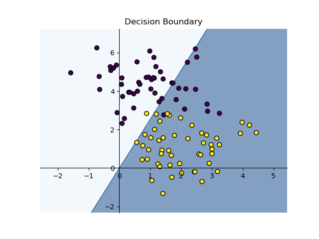
    # 训练前的决策边界
    estimator = MyPercetron()
    plot_decision_boundary(estimator, x, y)
    print('Acc:', estimator.score(x, y))

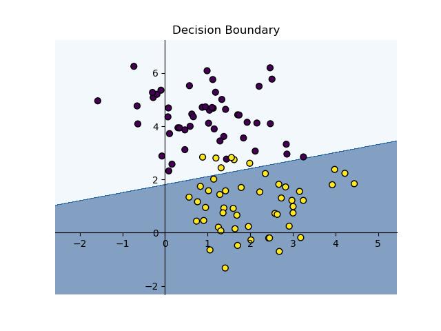
    # 训练后的决策边界
    estimator.fit(x, y)
    plot_decision_boundary(estimator, x, y)
    print('Acc:', estimator.score(x, y))


if __name__ == '__main__':
    test()

训练前（随机参数，左图）Acc: 0.796，训练前（右图）Acc: 0.956

3. 参数详解

from sklearn.datasets import make_blobs
import numpy as np
from sklearn.linear_model import Perceptron


def test():

    x, y = make_blobs(n_samples=1000, centers=2, n_features=2, random_state=0)
    estimator = Perceptron(
        penalty=None,
        alpha=0.0001,
        l1_ratio=0.15,
        fit_intercept=True,
        max_iter=1000,
        tol=1e-3,
        shuffle=True,
        verbose=0,
        eta0=1.0,
        n_jobs=None,
        random_state=0,
        early_stopping=False,
        validation_fraction=0.1,
        n_iter_no_change=5,
        class_weight=None,
        warm_start=False)

    estimator.fit(x, y)
    print('Acc:', estimator.score(x, y))


if __name__ == '__main__':
    test()

5.1 正则化参数

penalty : {'l2', 'l1', 'elasticnet'}, 默认值：None

控制正则化类型，即惩罚项（正则化项）。它有三个选择：
- 'l2'：L2 正则化（岭回归），即加入权重平方的惩罚项。
- 'l1'：L1 正则化（Lasso 回归），即加入权重绝对值的惩罚项。
- 'elasticnet'：弹性网正则化，是 L1 和 L2 正则化的混合，使用了比例参数 l1_ratio 来调整 L1 和 L2 的混合比例。

alpha : float, 默认值：0.0001

这是正则化项的常数系数，用来控制正则化的强度。它决定了惩罚项的权重。如果设置较大，正则化效果更强，可能导致过拟合问题的缓解；如果设置较小，正则化的效果较弱。

l1_ratio : float, 默认值：0.15

只有在 penalty='elasticnet' 时才会用到。它是弹性网正则化的混合参数，决定 L1 正则化与 L2 正则化的比例。l1_ratio=0 完全是 L2 正则化，l1_ratio=1 完全是 L1 正则化。0 <= l1_ratio <= 1 的值表示在 L1 和 L2 之间的加权混合。

5.2 训练相关参数

fit_intercept : bool, 默认值：True

是否计算截距（偏置项）。如果设为 False，则认为数据已经进行了中心化处理（即均值为 0）。如果设为 True，模型会估计截距。

max_iter : int, 默认值：1000

最大的迭代次数（即最大 epoch 数）。如果在这个次数内模型还没有收敛，训练会停止。对于感知机来说，可能导致训练较长时间，尤其是在数据复杂时。

tol : float or None, 默认值：1e-3

停止准则。训练将停止当 loss > previous_loss - tol，即如果损失值的变化小于该值，则停止训练。如果是 None，则不会使用停止准则。

shuffle : bool, 默认值：True

是否在每个 epoch 后打乱训练数据。通常，打乱数据有助于避免模型学习到数据的顺序特性，提高泛化能力。

eta0 : float, 默认值：1

更新时使用的初始学习率。学习率是训练过程中的重要参数，决定了模型参数更新的幅度。较高的学习率可能导致不收敛，较低的学习率可能导致训练时间过长。

class_weight : dict 或 "balanced", 默认值：None

为每个类别设置权重，可以使用 {class_label: weight} 的字典形式指定，也可以设置为 "balanced"，表示自动根据类别频率进行调整。通过 class_weight，可以平衡数据集中的类别不平衡问题，帮助模型更好地学习少数类。

warm_start : bool, 默认值：False

如果设置为 True，则会在调用 fit 时使用上次调用的模型参数作为初始化，而不是重新开始训练。这个参数通常用于增量学习，尤其在大数据或在线学习场景中。

5.3 训练控制参数

n_jobs : int, 默认值：None

并行计算时使用的 CPU 核心数。None 表示使用 1 个 CPU 核心，-1 表示使用所有可用的 CPU 核心。这个参数在多类别问题的 OVA（One vs All）训练中比较常见。

random_state : int, RandomState 实例或 None, 默认值：0

用于打乱训练数据的随机种子。如果设置了 random_state，则每次训练的结果是可重现的。

early_stopping : bool, 默认值：False

是否使用早停（Early Stopping）。当验证集的得分在多个 epoch 中没有改善时，训练将会停止。这个参数通常用于避免过拟合，尤其是在验证集上性能不再提升时。

validation_fraction : float, 默认值：0.1

如果使用 early_stopping=True，该参数控制从训练数据中抽取多少比例作为验证集。通常使用 10%（即 0.1）来评估模型在训练过程中的表现。

n_iter_no_change : int, 默认值：5

如果训练在连续 n_iter_no_change 次迭代中没有任何改进，训练会停止。这个参数与早停机制密切相关。

感知机（Perceptron）