


循环神经网络(Recurrent Neural Network, RNN)是一类用于处理序列数据的神经网络。
什么是序列数据?
序列数据是指按照一定顺序排列的数据集合,其中的每个元素被称为序列的一个项。序列数据可以是有限的,也可以是无限的。简言之:
- 每个元素都有一个位置,其位置对于理解和处理数据很重要。
- 序列数据中的元素之间可能存在依赖关系。
比如:我爱你、你爱我
1. 算法原理
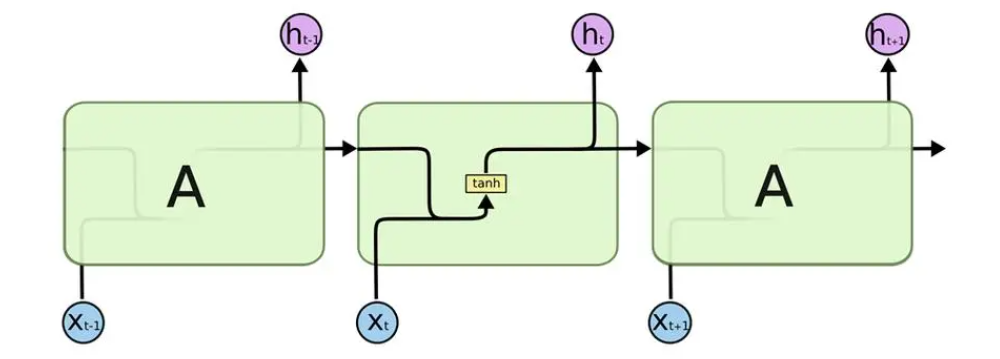
RNN 的基本思想是通过循环连接的方式使网络能够记住先前输入的信息,从而在处理当前输入时考虑到之前的信息。RNN 通过隐藏状态(hidden state)来存储之前时间步的信息,每次对输入的表示都会结合之前的信息来表示。
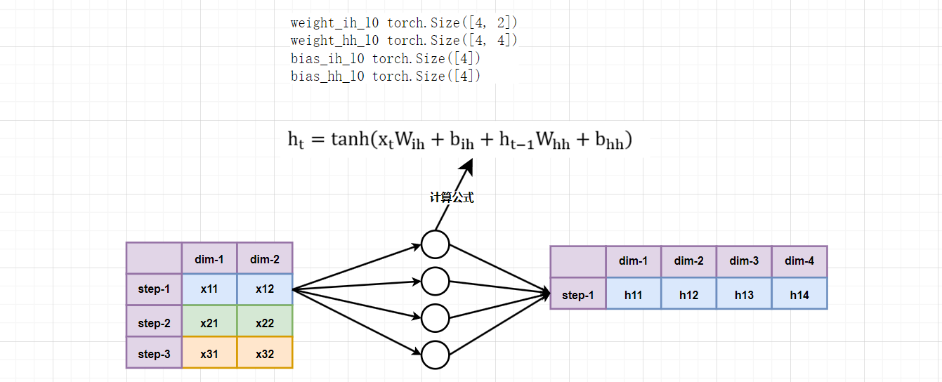
具体的计算公式如下:

- \(h_t\):在时间步 t 的隐藏状态向量
- \(h_{t-1}\):在时间步 t-1 的隐藏状态向量
- \(x_t\):在时间步 t 的输入向量
- \(W_{ih}\):输入 x 对应的权重矩阵
- \(b_{ih}\):输入 x 对应的偏置向量
- \(W_{hh}\):隐藏状态对应的权重矩阵
- \(b_{hh}\):隐藏状态对应的偏置向量
- \(tanh\):隐藏层激活函数
2. 算法使用
在 PyTorch 中,nn.RNNCell 和 nn.RNN 都用于构建循环神经网络(RNN),但它们的用途和适用场景有所不同。
2.1 nn.RNN
import torch
import torch.nn as nn
def test():
# 固定网络模型参数
torch.manual_seed(42)
# 1. 重点: 对象参数
# input_size 输入数据维度
# hidden_size 隐藏状态维度(神经元个数,输出数据维度)
rnn = nn.RNN(input_size=2, hidden_size=4, batch_first=False)
# 2. 重点: 输入
if rnn.batch_first:
# 构造输入(batch_size, seq_len, dim)
inputs = torch.rand(1, 3, 2)
else:
# 构造输入(seq_len, batch_size, dim)
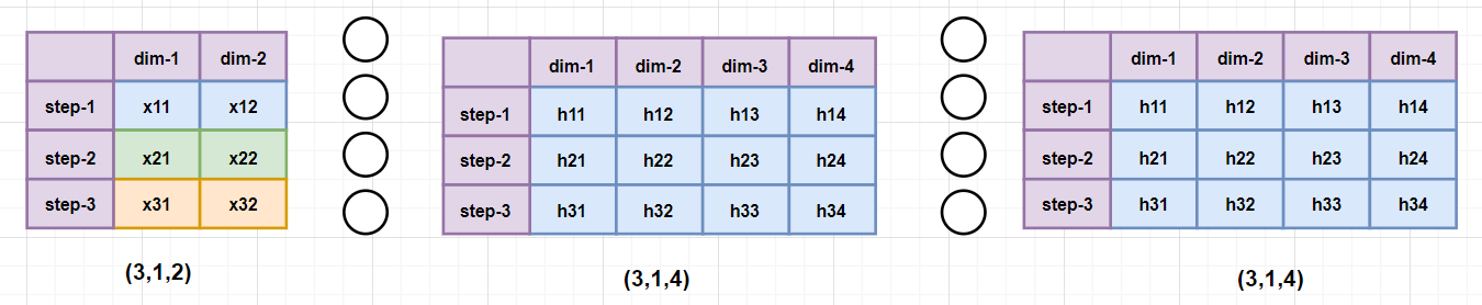
inputs = torch.rand(3, 1, 2)
# 3. 重点: 输出
# output 每个元素的隐藏状态
# hn 最后一个元素的隐藏状态
output, hn = rnn(inputs)
# output shape: torch.Size([3, 1, 4]) hn shape: torch.Size([1, 1, 4])
print('output shape:', output.shape, 'hn shape:', hn.shape)
# 4. 重点:参数量
# weight_ih_l0 torch.Size([4, 2])
# weight_hh_l0 torch.Size([4, 4])
# bias_ih_l0 torch.Size([4])
# bias_hh_l0 torch.Size([4])
for name, parameters in rnn.named_parameters():
print(name, parameters.size())
if __name__ == '__main__':
test()
2.2 num_players
num_layers 参数在 PyTorch 的 nn.RNN 模块中定义了堆叠在一起的 RNN 层的数量。每一层的隐藏状态将作为下一层的输入,从而使模型能够学习更复杂的表示和捕捉更高层次的特征。
单层 RNN 可能只能捕捉到输入序列的低级别特征。通过堆叠多层 RNN,可以逐层提取更加抽象和高级的特征,从而提高模型的表达能力和性能。
import torch
import torch.nn as nn


def test():
    torch.manual_seed(42)
    # num_layers 设置层数
    rnn = nn.RNN(input_size=2, hidden_size=4, num_layers=2)
    inputs = torch.rand(3, 1, 2)
    output, hn = rnn(inputs)
    print('output shape:', output.shape)
    print('hn shape:', hn.shape)
    print('-' * 30)
    for name, parameters in rnn.named_parameters():
        print(name, parameters.size())

if __name__ == '__main__':
    test()
程序输出结果:
output shape: torch.Size([3, 1, 4])
hn shape: torch.Size([2, 1, 4])
------------------------------
weight_ih_l0 torch.Size([4, 2])
weight_hh_l0 torch.Size([4, 4])
bias_ih_l0 torch.Size([4])
bias_hh_l0 torch.Size([4])
weight_ih_l1 torch.Size([4, 4])
weight_hh_l1 torch.Size([4, 4])
bias_ih_l1 torch.Size([4])
bias_hh_l1 torch.Size([4])
2.3 bidirectional
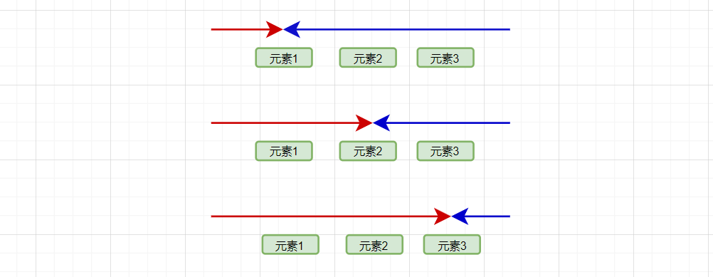
在很多自然语言处理(NLP)和序列处理任务中,当前时间步的输出不仅依赖于之前的时间步,还可能依赖于之后的时间步。
通过结合前向和后向的隐藏状态,双向 RNN 能够提供更丰富的上下文信息。这通常可以提高模型在各种任务上的表现,例如文本分类、命名实体识别和语言建模等。更多的信息通常意味着更准确的预测和更好的泛化性能。
在实现上,双向 RNN 包含两个独立的 RNN,一个处理正向序列(从前到后),一个处理反向序列(从后到前)。每个方向都有自己的一组权重参数。
import torch
import torch.nn as nn


def test():

    torch.manual_seed(42)
    rnn = nn.RNN(input_size=2, hidden_size=3, bidirectional=True)
    rnn_inputs = torch.rand(3, 1, 2)

    output, hn = rnn(rnn_inputs)

    # weight_ih_l0 torch.Size([3, 2])
    # weight_hh_l0 torch.Size([3, 3])
    # bias_ih_l0 torch.Size([3])
    # bias_hh_l0 torch.Size([3])
    # weight_ih_l0_reverse torch.Size([3, 2])
    # weight_hh_l0_reverse torch.Size([3, 3])
    # bias_ih_l0_reverse torch.Size([3])
    # bias_hh_l0_reverse torch.Size([3])
    for name, parameters in rnn.named_parameters():
        print(name, parameters.size())
    print('-' * 67)

    # output shape: torch.Size([3, 1, 6]) hn shape: torch.Size([2, 1, 3])
    print('output shape:', output.shape, 'hn shape:', hn.shape)
    print('-' * 67)

    print(output)
    print('-' * 67)

    print(hn)


if __name__ == '__main__':
    test()
程序输出结果:
weight_ih_l0 torch.Size([3, 2])
weight_hh_l0 torch.Size([3, 3])
bias_ih_l0 torch.Size([3])
bias_hh_l0 torch.Size([3])
weight_ih_l0_reverse torch.Size([3, 2])
weight_hh_l0_reverse torch.Size([3, 3])
bias_ih_l0_reverse torch.Size([3])
bias_hh_l0_reverse torch.Size([3])
-------------------------------------------------------------------
output shape: torch.Size([3, 1, 6]) hn shape: torch.Size([2, 1, 3])
-------------------------------------------------------------------
tensor([[[ 0.3936,  0.7608, -0.1589, -0.0829,  0.1864, -0.5768]],

        [[ 0.1960,  0.6819, -0.0645,  0.1314,  0.1977, -0.5505]],

        [[ 0.3993,  0.7820, -0.0925, -0.2763,  0.5750, -0.3795]]],
       grad_fn=<CatBackward0>)
-------------------------------------------------------------------
tensor([[[ 0.3993,  0.7820, -0.0925]],

        [[-0.0829,  0.1864, -0.5768]]], grad_fn=<StackBackward0>)
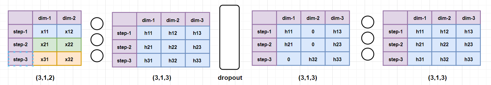
2.4 dropout
dropout 参数表示的是一种正则化技术,用于防止神经网络的过拟合。过拟合是指模型在训练数据上表现很好,但在测试数据上表现不佳,原因是模型过于复杂,学到了训练数据中的噪声。
Dropout 的基本思想是在训练过程中,随机将一部分神经元的输出设为零,从而减少神经元之间的相互依赖。这在训练过程中强制模型学习更加鲁棒的特征。
在 nn.RNN 中,如果设置了非零的 dropout 参数值,那么在每一层 RNN(循环神经网络)的输出之后(除了最后一层),都会添加一个 Dropout 层。
该 Dropout 层的概率等于 dropout 参数的值。例如,如果 dropout=0.5,那么每一层 RNN 输出的神经元有 50% 的概率被设置为零。
默认情况下,dropout 参数是 0,意味着不使用 Dropout。
import torch
import torch.nn as nn


def test():
    torch.manual_seed(42)
    rnn = nn.RNN(input_size=2, hidden_size=3, dropout=0.2, num_layers=2)
    rnn_inputs = torch.rand(3, 1, 2)
    output, hn = rnn(rnn_inputs)
    print(hn)


if __name__ == '__main__':
    test()
2.5 RNNCell
nn.RNNCell 代表单个时间步的 RNN 单元,它用于需要对每个时间步手动进行处理的场景。适合高级用户或需要对 RNN 的时间步迭代进行细粒度控制的场景。使用 nn.RNNCell 可以更灵活地操作隐藏状态,适合构建自定义的 RNN 结构或在循环体中嵌入其他操作。
import torch
import torch.nn as nn


def test01():
    # 固定网络模型参数
    torch.manual_seed(42)
    # input_size 输入数据维度
    # hidden_size 隐藏状态维度(神经元个数,输出数据维度)
    rnn = nn.RNN(input_size=4, hidden_size=6)
    # 构造输入(seq_len, batch_size, dim)
    rnn_inputs = torch.rand(3, 2, 4)
    output, hn = rnn(rnn_inputs)

    # 输出结果
    print(output.squeeze())
    print(hn)


def test02():
    # 固定网络模型参数
    torch.manual_seed(42)

    # input_size 输入数据维度
    # hidden_size 神经元数量(输出维度)
    rnn = nn.RNNCell(input_size=4, hidden_size=6)
    # 构造输入(seq_len, batch_size, dim)
    rnn_inputs = torch.rand(3, 2, 4)
    # 初始化隐藏状态(每个序列分别初始化隐藏状态)
    rnn_hidden = torch.zeros(2, 6)
    # 保存隐藏状态
    hidden_states = []

    # 训练计算时间隐藏状态
    for idx in range(rnn_inputs.shape[0]):
        rnn_hidden = rnn(rnn_inputs[idx], rnn_hidden)
        hidden_states.append(rnn_hidden)

    output = torch.stack(hidden_states)
    hn = rnn_hidden

    # 输出结果
    print(output)
    print(hn)

if __name__ == '__main__':
    test01()
    print('-' * 30)
    test02()
程序输出结果:
tensor([[[ 0.6295, -0.5197,  0.2157, -0.0886,  0.6734, -0.1085],
         [ 0.7314, -0.3738,  0.0418, -0.2117,  0.5020,  0.1213]],

        [[ 0.4572, -0.2470,  0.1893, -0.0327,  0.3821,  0.2097],
         [ 0.5103, -0.3171,  0.3264,  0.1896,  0.6496, -0.0635]],

        [[ 0.5079, -0.2033, -0.0015, -0.0311,  0.5142,  0.0714],
         [ 0.6826, -0.1805, -0.0191,  0.0802,  0.5302,  0.1724]]],
       grad_fn=<SqueezeBackward0>)
tensor([[[ 0.5079, -0.2033, -0.0015, -0.0311,  0.5142,  0.0714],
         [ 0.6826, -0.1805, -0.0191,  0.0802,  0.5302,  0.1724]]],
       grad_fn=<StackBackward0>)
------------------------------
tensor([[[ 0.6295, -0.5197,  0.2157, -0.0886,  0.6734, -0.1085],
         [ 0.7314, -0.3738,  0.0418, -0.2117,  0.5020,  0.1213]],

        [[ 0.4572, -0.2470,  0.1893, -0.0327,  0.3821,  0.2097],
         [ 0.5103, -0.3171,  0.3264,  0.1896,  0.6496, -0.0635]],

        [[ 0.5079, -0.2033, -0.0015, -0.0311,  0.5142,  0.0714],
         [ 0.6826, -0.1805, -0.0191,  0.0802,  0.5302,  0.1724]]],
       grad_fn=<StackBackward0>)
tensor([[ 0.5079, -0.2033, -0.0015, -0.0311,  0.5142,  0.0714],
        [ 0.6826, -0.1805, -0.0191,  0.0802,  0.5302,  0.1724]],
       grad_fn=<TanhBackward0>)
 冀公网安备13050302001966号