在构建和训练分类模型之后，我们需要了解它的预测能力。简单地说，我们需要知道模型在处理新的未见过的数据时，是否能够准确地进行分类。通过性能评估，我们可以确定模型的优点和缺陷，进而指导我们对模型的改进和优化。

pip install scikit-learn -i https://pypi.tuna.tsinghua.edu.cn/simple/
pip install pandas -i https://pypi.tuna.tsinghua.edu.cn/simple/

接下来，我们了解下在不同的分类模型中，如何进行性能指标的计算和度量。

1. 二分类场景

1.1 准确率

对分类模型的性能评估时经常使用准确率（Accuracy）评估方法，准确率是指分类模型正确预测的样本数量与总样本数量之比。

例如：

假设：样本中有 6 个恶性肿瘤样本，4 个良性肿瘤样本。
模型 A：预测对了 5 个恶性肿瘤样本，4 个良性肿瘤样本，其准确率为：90%
模型 B：预测对了 6 个恶性肿瘤样本，3 个良性肿瘤样本，其准确率为：90%

from sklearn.metrics import accuracy_score
import pandas as pd


if __name__ == '__main__':
    # 样本集中共有6个恶性肿瘤样本, 4个良性肿瘤样本
    y_true = ['恶性', '恶性', '恶性', '恶性', '恶性', '恶性', '良性', '良性', '良性', '良性']

    # 1. 模型 A: 预测对了 5 个恶性肿瘤样本, 4个良性肿瘤样本
    y_pred = ['恶性', '恶性', '恶性', '恶性', '恶性', '良性', '良性', '良性', '良性', '良性']
    acc = accuracy_score(y_true, y_pred)
    print('acc:', acc)

    # 2. 模型 B: 预测对了 6 个恶性肿瘤样本, 3 个良性肿瘤样本
    y_pred = ['恶性', '恶性', '恶性', '恶性', '恶性', '恶性', '恶性', '良性', '良性', '良性']
    acc = accuracy_score(y_true, y_pred)
    print('acc:', acc)

acc: 0.9
acc: 0.9

1.2 混淆矩阵

准确率是一个较为粗粒度的分类评估方法，它并不能进行更加细粒度的评估场景。例如：在一个肿瘤预测的二分类问题中，我们更加看重模型对恶性肿瘤的预测能力，而不仅仅是准确率。模型 B 把所有潜在的恶性肿瘤患者全部预测出来，模型 A 只能把 5/6 的恶性肿瘤患者预测出来，哪一个模型对于当前问题场景更好呢？显然是前者。

所以，所以，我们需要引入其他的模型评估方法。

想要获得更加精细的分类评估方法，得将预测结果进行更为精细的划分，这就是混淆矩阵（Confusion Matrix）。

	正例（预测结果）	负例（预测结果）
正例（真实结果）	真正例（TP）	假负例（FN）
负例（真实结果）	假正例（FP）	真负例（TN）

混淆矩阵作用就是统计下在测试集中：

真实值是正例的样本中，被预测为正例的样本数量有多少，这部分样本叫做 真正例（TP，True Positive）
真实值是正例的样本中，被预测为负例的样本数量有多少，这部分样本叫做 假负例（FN，False Negative）
真实值是负例的样本中，被预测为正例的样本数量有多少，这部分样本叫做 假正例（FP，False Positive）
真实值是负例的样本中，被预测为负例的样本数量有多少，这部分样本叫做 真负例（TN，True Negative）

True Positive ：整体表示样本真实的类别
Positive ：第二个词表示样本被预测为的类别

例子：

样本集中有 6 个恶性肿瘤样本，4 个良性肿瘤样本，我们假设恶性肿瘤为正例，则：

模型 A：预测对了 3 个恶性肿瘤样本，4 个良性肿瘤样本
1. 真正例 TP 为：3
2. 假负例 FN 为：3
3. 假正例 FP 为：0
4. 真负例 TN：4
模型 B：预测对了 6 个恶性肿瘤样本，1个良性肿瘤样本
1. 真正例 TP 为：6
2. 假负例 FN 为：0
3. 假正例 FP 为：3
4. 真负例 TN：1

我们会发现：TP+FN+FP+TN = 总样本数量

通过上面四种情况，将预测后的结果划分为 4 部分，分别是：TP、FN、TN、FP。我们通过上述 4 种信息，构成了分类问题中的重要评估指标。

from sklearn.metrics import confusion_matrix
import pandas as pd


if __name__ == '__main__':
    # 样本集中共有6个恶性肿瘤样本, 4个良性肿瘤样本
    y_true = ['恶性', '恶性', '恶性', '恶性', '恶性', '恶性', '良性', '良性', '良性', '良性']

    labels = ['恶性', '良性']

    # 1. 模型 A: 预测对了3个恶性肿瘤样本, 4个良性肿瘤样本
    y_pred = ['恶性', '恶性', '恶性', '良性', '良性', '良性', '良性', '良性', '良性', '良性']
    matrix = confusion_matrix(y_true, y_pred, labels=labels)
    print(pd.DataFrame(matrix, columns=labels, index=labels))

    # 2. 模型 B: 预测对了6个恶性肿瘤样本, 1个良性肿瘤样本
    y_pred = ['恶性', '恶性', '恶性', '恶性', '恶性', '恶性', '恶性', '恶性', '恶性', '良性']
    matrix = confusion_matrix(y_true, y_pred, labels=labels)
    print(pd.DataFrame(matrix, columns=labels, index=labels))

    恶性  良性
恶性   3   3
良性   0   4

    恶性  良性
恶性   6   0
良性   3   1

1.3 精确率

精确率（Precision）是指被分类器正确分类的正样本（True Positive）数目与所有被分类为正样本的样本数目的比率。

比如，我们把恶性肿瘤当做正例样本，我们希望知道在模型预测出的所有的恶性肿瘤样本中，真正的恶性肿瘤样本占比。即：模型对恶性肿瘤的预测精确率有多少？

如果预测出 10 个恶性肿瘤样本，并且这 10 个也是真正的恶性肿瘤，那么精度就是 100%。如果 10 个中，只有 3 个是真正的恶性肿瘤，那么精度就是 30%.

也就是说，我们关心模型预测的准不准，并不关心预测的全不全。

例子：

样本集中有 6 个恶性肿瘤样本，4 个良性肿瘤样本，我们假设恶性肿瘤为正例，则：

模型 A：预测对了 3 个恶性肿瘤样本，4 个良性肿瘤样本
1. 真正例 TP 为：3
2. 假负例 FN 为：3
3. 假正例 FP 为：0
4. 真负例 TN：4
5. 精确率：3/(3+0) = 100%
模型 B：预测对了 6 个恶性肿瘤样本，1个良性肿瘤样本
1. 真正例 TP 为：6
2. 假负例 FN 为：0
3. 假正例 FP 为：3
4. 真负例 TN：1
5. 精确率：6/(6+3) = 67%

from sklearn.metrics import precision_score


if __name__ == '__main__':
    # 样本集中共有6个恶性肿瘤样本, 4个良性肿瘤样本
    y_true = ['恶性', '恶性', '恶性', '恶性', '恶性', '恶性', '良性', '良性', '良性', '良性']

    # 1. 模型 A: 预测对了3个恶性肿瘤样本, 4个良性肿瘤样本
    y_pred = ['恶性', '恶性', '恶性', '良性', '良性', '良性', '良性', '良性', '良性', '良性']

    # pos_label 指定那个类别是正例
    result = precision_score(y_true, y_pred, pos_label='恶性')
    print('模型A精确率:', result)

    # 2. 模型 B: 预测对了6个恶性肿瘤样本, 1个良性肿瘤样本
    y_pred = ['恶性', '恶性', '恶性', '恶性', '恶性', '恶性', '恶性', '恶性', '恶性', '良性']

    result = precision_score(y_true, y_pred, pos_label='恶性')
    print('模型B精确率:', result)

输出结果：

模型A精确率: 1.0
模型B精确率: 0.67

1.4 召回率

召回率也叫做查全率，指的是预测为真正例样本占所有真实正例样本的比重。例如：我们把恶性肿瘤当做正例样本，则我们想知道模型是否能把所有的恶性肿瘤患者都预测出来。

例子：

样本集中有 6 个恶性肿瘤样本，4 个良性肿瘤样本，我们假设恶性肿瘤为正例，则：

模型 A：预测对了 3 个恶性肿瘤样本，4 个良性肿瘤样本
1. 真正例 TP 为：3
2. 假负例 FN 为：3
3. 假正例 FP 为：0
4. 真负例 TN：4
5. 精确率：3/(3+0) = 100%
6. 召回率：3/(3+3)=50%
模型 B：预测对了 6 个恶性肿瘤样本，1个良性肿瘤样本
1. 真正例 TP 为：6
2. 假负例FN 为：0
3. 假正例 FP 为：3
4. 真负例 TN：1
5. 精确率：6/(6+3) = 67%
6. 召回率：6/(6+0)= 100%

from sklearn.metrics import recall_score


if __name__ == '__main__':

    # 样本集中共有6个恶性肿瘤样本, 4个良性肿瘤样本
    y_true = ['恶性', '恶性', '恶性', '恶性', '恶性','恶性', '良性', '良性', '良性', '良性']

    # 1. 模型 A: 预测对了3个恶性肿瘤样本, 4个良性肿瘤样本
    y_pred = ['恶性', '恶性', '恶性', '良性', '良性', '良性', '良性', '良性', '良性', '良性']

    result = recall_score(y_true, y_pred, pos_label='恶性')
    print('模型A召回率:', result)


    # 2. 模型 B: 预测对了6个恶性肿瘤样本, 1个良性肿瘤样本
    y_pred = ['恶性', '恶性', '恶性', '恶性', '恶性', '恶性', '恶性', '恶性', '恶性', '良性']

    result = recall_score(y_true, y_pred, pos_label='恶性')
    print('模型B召回率:', result)

输出结果：

模型A召回率: 0.5
模型B召回率: 1.0

1.5 F1-score

F1-score 是一种常用的性能度量指标，它综合考虑了模型的精确度和召回率，是这两者的调和平均数，其计算公式如下：

调和平均数对数据集中的较小数值更敏感。如果数据集中有极小的值，它会显著降低调和平均数的值。

from scipy.stats import hmean


print(hmean([0.0, 1.0]))
print(hmean([1.0, 0.0]))
print(hmean([0.0, 0.0]))
print(hmean([1.0, 1.0]))

0.0
0.0
0.0
1.0

所以，当精度和召回率都高的时候，f1-score 才会高。

样本集中有 6 个恶性肿瘤样本，4 个良性肿瘤样本，我们假设恶性肿瘤为正例，则：

模型 A：预测对了 3 个恶性肿瘤样本，4 个良性肿瘤样本
1. 真正例 TP 为：3
2. 假负例 FN 为：3
3. 假正例 FP 为：0
4. 真负例 TN：4
5. 精确率：3/(3+0) = 100%
6. 召回率：3/(3+3)=50%
7. F1-score：(2*3)/(2*3+3+0)=67%
模型 B：预测对了 6 个恶性肿瘤样本，1个良性肿瘤样本
1. 真正例 TP 为：6
2. 假负例 FN 为：0
3. 假正例 FP 为：3
4. 真负例 TN：1
5. 精确率：6/(6+3) = 67%
6. 召回率：6/(6+0)= 100%
7. F1-score：(2*6)/(2*6+0+3)=80%

from sklearn.metrics import f1_score


if __name__ == '__main__':

    # 样本集中共有6个恶性肿瘤样本, 4个良性肿瘤样本
    y_true = ['恶性', '恶性', '恶性', '恶性', '恶性','恶性', '良性', '良性', '良性', '良性']

    # 1. 模型 A: 预测对了3个恶性肿瘤样本, 4个良性肿瘤样本
    y_pred = ['恶性', '恶性', '恶性', '良性', '良性', '良性', '良性', '良性', '良性', '良性']
    
    result = f1_score(y_true, y_pred, pos_label='恶性')
    print('模型A f1-score:', result)


    # 2. 模型 B: 预测对了6个恶性肿瘤样本, 1个良性肿瘤样本
    y_pred = ['恶性', '恶性', '恶性', '恶性', '恶性', '恶性', '恶性', '恶性', '恶性', '良性']

    result = f1_score(y_true, y_pred, pos_label='恶性')
    print('模型B f1-score:', result)

输出结果：

模型A f1-score: 0.67
模型B f1-score: 0.8

2. 多分类场景

在评估多分类模型性能时，我们经常会使用一些指标来衡量其表现。其中，micro-averaging、macro-averaging 和 weighted-averaging 是常见的评估指标之一。它们在衡量分类器的精确度、召回率和 F1 分数时发挥着重要作用。

假设：三分类的真实标签和预测标签如下：

y_true = ['好评', '好评', '好评', '中评', '中评', '差评', '差评', '差评', '差评', '差评']
y_pred = ['好评', '好评', '好评', '好评', '中评', '差评', '好评', '中评', '差评', '中评']

对应的混淆矩阵：

    好评  中评  差评
好评   3   0   0
中评   1   1   0
差评   1   2   2

每个类别的评估分数：

精确率:		 [0.6        0.33333333      1.        ]
召回率:		 [1.         0.5             0.4       ]
f1-score:	 [0.75       0.4             0.57142857]

from sklearn.metrics import precision_score
from sklearn.metrics import recall_score
from sklearn.metrics import f1_score
from sklearn.metrics import confusion_matrix
import pandas as pd


if __name__ == '__main__':

    y_true = ['好评', '好评', '好评', '中评', '中评', '差评', '差评', '差评', '差评', '差评']
    y_pred = ['好评', '好评', '好评', '好评', '中评', '差评', '好评', '中评', '差评', '中评']

    # 混淆矩阵
    labels = ['好评', '中评', '差评']
    matrix = confusion_matrix(y_true, y_pred, labels=labels)
    matrix = pd.DataFrame(matrix, columns=labels, index=labels)
    print(matrix)
    print()

    # 返回所有类别分数
    result = precision_score(y_true, y_pred, average=None, labels=['好评', '中评', '差评'])
    print('精确率:\t\t', result)

    result = recall_score(y_true, y_pred, average=None, labels=['好评', '中评', '差评'])
    print('召回率:\t\t', result)

    result = f1_score(y_true, y_pred, average=None, labels=['好评', '中评', '差评'])
    print('f1-score:\t', result)

2.1 micro-averaging

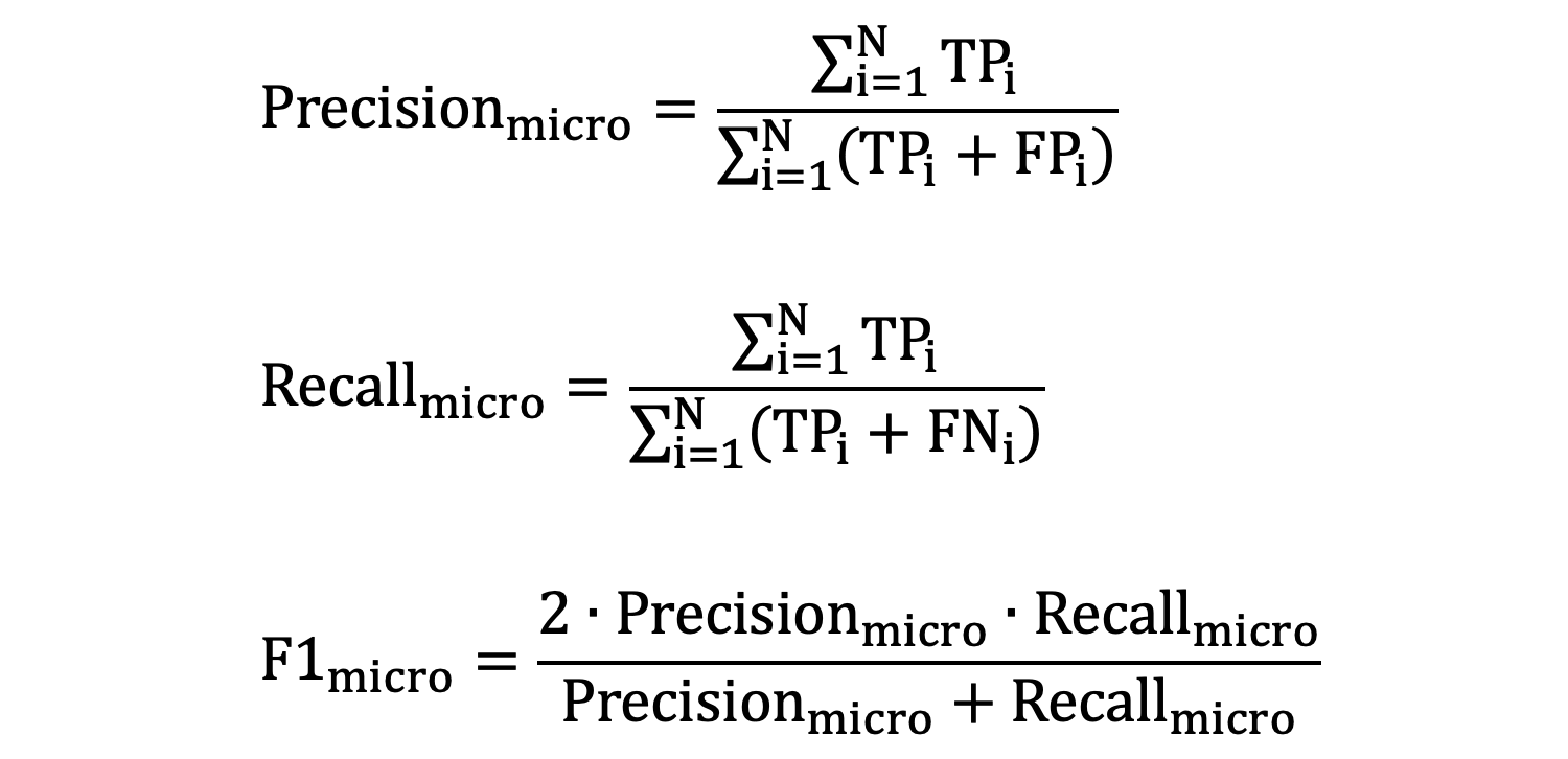
\(N\) 是类别总数
\(TP_{i}\) 是第 𝑖 个类别的 TP 之和
\(FP_{i}\) 是第 𝑖 个类别的 FP 之和
\(FN_{i}\)是第 𝑖 个类别的 FN 之和

我们以前面例子为例：

好评：
TP = 3 （预测为好评且实际为好评）
FP = 1+1 = 2 （预测为好评但实际为中评和差评）
TN = 1+2+2 = 5 （预测不是好评且实际也不是好评，包括中评和差评）
FN = 0+0 = 0 （实际为好评但预测不是好评）

中评：
TP = 1 （预测为中评且实际为中评）
FP = 0+2 = 2 （预测为中评但实际为好评和差评）
TN = 3+2+1+0 = 6 （预测不是中评且实际也不是中评，包括好评和差评）
FN = 1+0 = 1 （实际为中评但预测不是中评）

差评：
TP = 2 （预测为差评且实际为差评）
FP = 0+0 = 0 （没有将其他类别预测为差评）
TN = 3+1+1 = 5 （预测不是差评且实际也不是差评，包括好评和中评）
FN = 1+2 = 3 （实际为差评但预测不是差评）


每个类别的 TP、FP、TN、FN 值分别是：
好评：TP=3, FP=2, TN=5, FN=0
中评：TP=1, FP=2, TN=6, FN=1
差评：TP=2, FP=0, TN=6, FN=3


此时：
TP = 3 + 1 + 2 = 6
FP = 2 + 2 + 0 = 4
TN = 5 + 7 + 6 = 18
FN = 0 + 1 + 3 = 4

使用上述计算得到的 TP、FP、TN、FN 值：

micro-averaged precision：TP/(TP+FP) = 6/(6+4) = 0.6
micro-averaged recall：TP/(TP+FN) = 6/(6+4) = 0.6
micro-averaged f1-score：2*(micro-averaged precision * micro-averaged recall) / (micro-averaged precision+micro-averaged recall) = 2*(0.6*0.6)/(0.6+0.6) = 0.6

from sklearn.metrics import precision_score
from sklearn.metrics import recall_score
from sklearn.metrics import f1_score


if __name__ == '__main__':

    y_true = ['好评', '好评', '好评', '中评', '中评', '差评', '差评', '差评', '差评', '差评']
    y_pred = ['好评', '好评', '好评', '好评', '中评', '差评', '好评', '中评', '差评', '中评']

    result = precision_score(y_true, y_pred, average='micro')
    print('精确率:\t\t', result)

    result = recall_score(y_true, y_pred, average='micro')
    print('召回率:\t\t', result)

    result = f1_score(y_true, y_pred, average='micro')
    print('f1-score:\t', result)

精确率:		 0.6
召回率:		 0.6
f1-score:	 0.6

2.2 macro-averaging

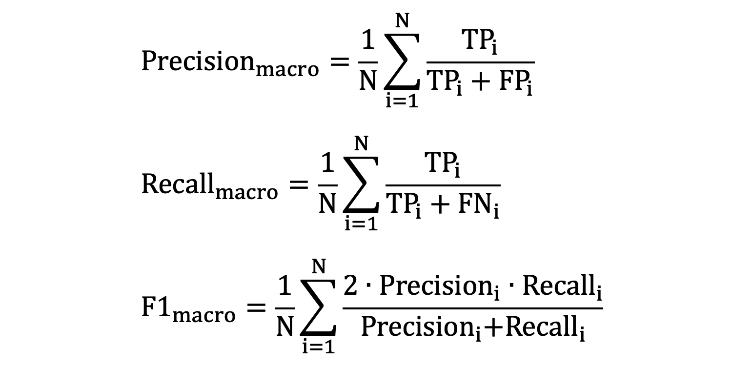
macro-averaging 计算每个类别的精确度、召回率和 F1 分数，然后对它们取算术平均值。

好评：
精确率：0.6
召回率：1.0
f1-score：0.75


中评：
精确率：0.33
召回率：0.5
f1-score：0.4


差评：
精确率：1
召回率：0.4
f1-score：0.57

macro-averaged precision: (0.6 + 0.33 + 1) / 3 = 0.64
macro-averaged recall：(1.0 + 0.5 + 0.4) / 3 = 0.63
macro-averaged f1-score：(0.75 + 0.4 + 0.57) / 3 = 0.57

from sklearn.metrics import precision_score
from sklearn.metrics import recall_score
from sklearn.metrics import f1_score


if __name__ == '__main__':

    y_true = ['好评', '好评', '好评', '中评', '中评', '差评', '差评', '差评', '差评', '差评']
    y_pred = ['好评', '好评', '好评', '好评', '中评', '差评', '好评', '中评', '差评', '中评']

    result = precision_score(y_true, y_pred, average='macro')
    print('精确率:\t\t', result)

    result = recall_score(y_true, y_pred, average='macro')
    print('召回率:\t\t', result)

    result = f1_score(y_true, y_pred, average='macro')
    print('f1-score:\t', result)

精确率:		 0.6444444444444445
召回率:		 0.6333333333333333
f1-score:	 0.5738095238095239

2.3 weighted-averaging

假设：共有 100 个样本：

好评：70，精度为：0.3
中评：20，精度为：0.6
差评：10，精度为：0.9

宏平均 = (0.3 + 0.6 + 0.9) / 3 = 0.6

在大多数样本上，模型只有 0.3 的精度，但是宏平均的精度却达到了 0.6。所以，宏平均不能真实的反映出模型在大多数样本上的表现。

weighted-averaging 计算每个类别的精确度、召回率和 F1 分数，然后将它们乘以每个类别的样本数或权重，最后将所有类别的加权平均值。它能够反应出样本在大多数样本上的表现。

加权平均：0.3 * 0.7 + 0.6 * 0.2 + 0.9 * 0.1 = 0.42，由此可以看到加权平均更加能够反映出模型在大多数样本上的表现。

接着前面的例子：

由 y_true = ['好评', '好评', '好评', '中评', '中评', '差评', '差评', '差评', '差评', '差评']
可知每个类别的权重分别为：0.3、0.2、0.5

weighted-averaged precision：0.6 * 0.3 + 0.33 * 0.2 + 1 * 0.5 = 0.746
weighted-averaged recall：1 * 0.3 + 0.5 * 0.2 + 0.4 * 0.5 = 0.6
weighted-averaged f1-score：0.75 * 0.3 + 0.4 * 0.2 + 0.57 * 0.5 = 0.59

from sklearn.metrics import precision_score
from sklearn.metrics import recall_score
from sklearn.metrics import f1_score


if __name__ == '__main__':

    y_true = ['好评', '好评', '好评', '中评', '中评', '差评', '差评', '差评', '差评', '差评']
    y_pred = ['好评', '好评', '好评', '好评', '中评', '差评', '好评', '中评', '差评', '中评']

    result = precision_score(y_true, y_pred, average='weighted')
    print('精确率:\t\t', result)

    result = recall_score(y_true, y_pred, average='weighted')
    print('召回率:\t\t', result)

    result = f1_score(y_true, y_pred, average='weighted')
    print('f1-score:\t', result)

精确率:		 0.7466666666666667
召回率:		 0.6
f1-score:	 0.5907142857142857

3. 多标签场景

多标签分类是指每个样本可以被分配到多个类别中，即：可以拥有多个标签。比如：某条新闻既可以是军事类新闻、也可以是政治类新闻。

在评估多标签分类模型时，我们使用的是样本平均精确率、样本平均召回率和样本平均 F1 分数。

y_true = [['好评', '中评'], ['好评', '中评', '差评'], ['好评', '差评'], ['中评', '差评'], ['中评', '好评']]
y_pred = [['中评', ], ['好评', '差评'], ['中评', ], ['好评', '差评'], ['中评', '好评']]

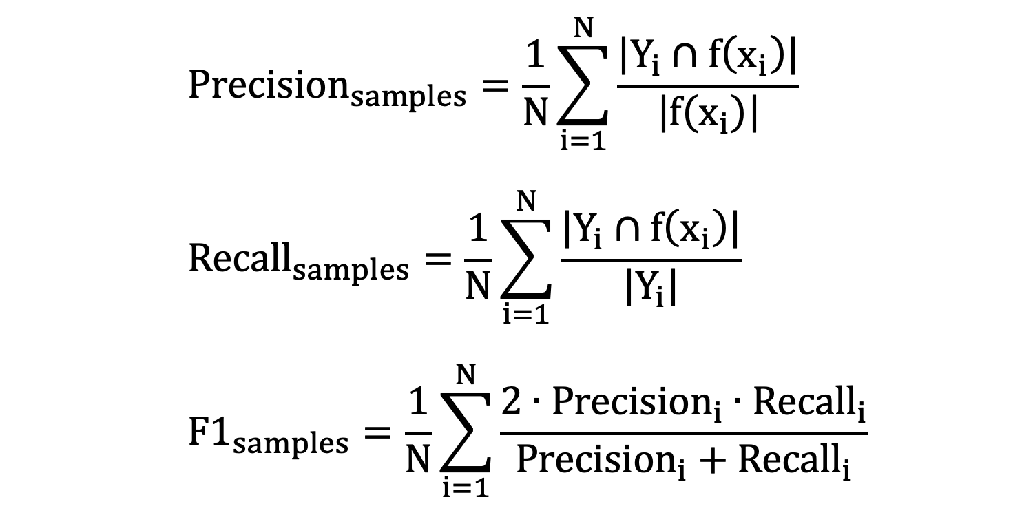
\(N\) 表示样本数量
\(Y_{i}\) 表示第 i 个样本真实标签集合
\(f(x_{i})\) 表示第 i 个样本预测的标签集合
\(Precision_{i}\) 表示第 i 个样本的精确度
\(Recall_{i}\) 表示第 i 个样本的召回率

接下来，计算每个样本的精确度、召回率、f1-score 值如下:

样本1：
精确度：1.0 
召回率：0.5 
F1-score：0.6666666666666666

样本2：
精确度：1.0 
召回率：0.6666666666666666 
F1-score：0.8

样本3：
精确度：0.0 
召回率：0.0 
F1-score：0.0

样本4：
精确度：0.5 
召回率：0.5 
F1-score：0.5

样本5：
精确度：1.0 
召回率：1.0 
F1-score：1.0

计算每个指标的样本平均值：

精确度：0.7
召回率：0.5333333333333333
F1-score：0.5933333333333334

使用示例：

from sklearn.metrics import precision_score
from sklearn.metrics import recall_score
from sklearn.metrics import f1_score
from sklearn.preprocessing import MultiLabelBinarizer
import pandas as pd


if __name__ == '__main__':

    # 真实和预测标签
    y_true = [['好评', '中评'],  ['好评', '中评', '差评'], ['好评', '差评'], ['中评', '差评'], ['中评', '好评']]
    y_pred = [['中评', ], ['好评', '差评'], ['中评', ], ['好评', '差评'], ['中评', '好评']]

    # 注意：必须对标签进行重新编码
    mlb = MultiLabelBinarizer()
    y_true = mlb.fit_transform(y_true)
    y_pred = mlb.transform(y_pred)
    print(mlb.classes_)
    print(y_true)
    print(y_pred)

    result = precision_score(y_true, y_pred, average='samples')
    print('精确率:\t\t', result)

    result = recall_score(y_true, y_pred, average='samples')
    print('召回率:\t\t', result)

    result = f1_score(y_true, y_pred, average='samples')
    print('f1-score:\t', result)

['中评' '好评' '差评']
[[1 1 0]
 [1 1 1]
 [0 1 1]
 [1 0 1]
 [1 1 0]]
[[1 0 0]
 [0 1 1]
 [1 0 0]
 [0 1 1]
 [1 1 0]]
精确率:		 0.7
召回率:		 0.5333333333333333
f1-score:	 0.5933333333333334

分类性能评估方法

1. 二分类场景

1.1 准确率

1.2 混淆矩阵

1.3 精确率

1.4 召回率

1.5 F1-score

2. 多分类场景

2.1 micro-averaging

2.2 macro-averaging

2.3 weighted-averaging

3. 多标签场景

取消回复

文章目录