《GBDT 梯度提升树》多分类过程

GBDT（Gradient Boosting Decision Tree，梯度提升树）本质上是一个 二分类模型。它通过不断迭代地拟合前一轮模型的“残差”（即负梯度），逐步提升模型的预测精度。在二分类任务中，GBDT 结合 Sigmoid 函数 输出类别概率。

然而，在实际任务中，我们经常会遇到多分类问题（如三分类、五分类等）。GBDT 并不能直接处理多类别标签，因此需要借助一种常见的扩展策略：OVR（One-vs-Rest，一对多），OVR 思想如下：

假设训练数据中有 K 个类别（例如：0、1、2），那么我们就训练 K 个独立的二分类 GBDT 模型：

模型 0：用于区分类别 0 和非 0 类
模型 1：用于区分类别 1 和非 1 类
模型 2：用于区分类别 2 和非 2 类

在预测时，将样本分别送入这 K 个模型中，得到 K 个分数，这 K 个分数就表示该样本属于不同类别的分数，最后使用 Softmax 函数 将这些分数归一化为概率：

接下来，我们通过一个具体的计算案例来加深对 GBDT 应用多分类过程的理解。

假设：数据集中有 20 条数据， 50% 为 0 标签，30% 为 1 标签，20% 为 2 标签。接下来使用 GBDT 预测新样本：[0.49671415 -0.1382643 0.64768854] 的类别标签。

每个 GBDT 模型在训练前都有一个初始分数，这个分数反映了类别的先验概率。由于多分类使用 Softmax 函数（二分类使用的是 sigmoid 函数），因此初始分数可通过对数计算：

代入数据得到：

类别	占比 (\(p_{k}\))	初始分数(\(F_{k}^{0}\))
0	0.5	-0.6931471805599453
1	0.3	-1.2039728043259361
2	0.2	-1.6094379124341003

由于是多分类，GBDT 得到的模型结构（3 个二分类 GBDT 分类器）如下：

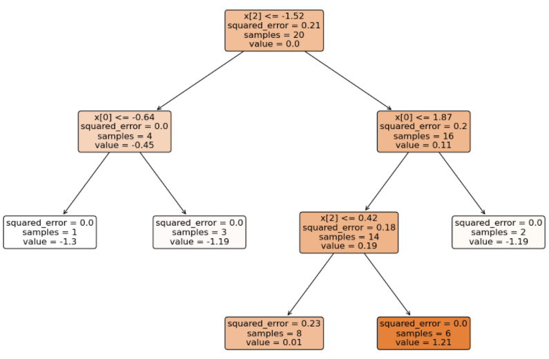
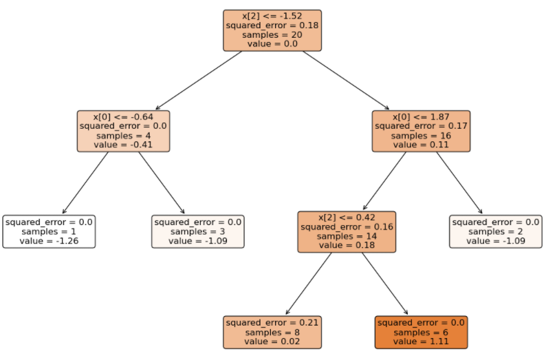
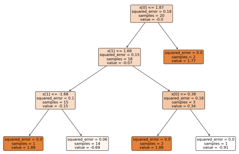
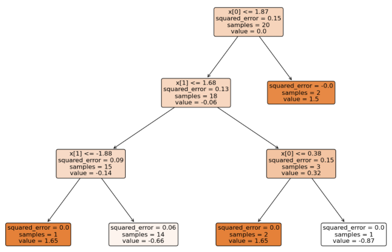
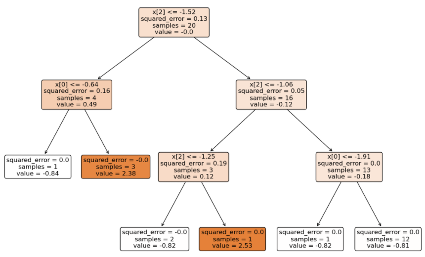
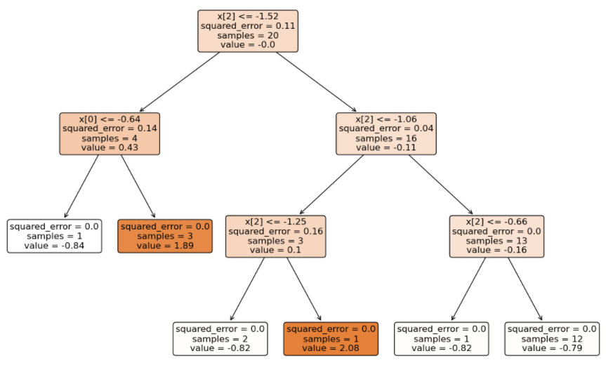
将待预测的样本分别输入到不同类别的 GBDT 中得到分数（学习率 0.1）：

输入到 0 类别 GBDT 得到的分数总和：(1.33 + 1.21 + 1.11) * 0.1 = 0.365
输入到 1 类别 GBDT 得到的分数总和：(-0.73 – 0.69 – 0.66) * 0.1 = -0.208
输入到 2 类别 GBDT 得到的分数总和：(-0.83 – 0.81 – 0.79) * 0.1 = -0.243

再分别加上属于不同类别的初始分数：

属于 0 类别分数：-0.6931471805599453 + 0.365 = -0.3281471805599453
属于 1 类别分数：-1.2039728043259361 – 0.208 = -1.411972804325936
属于 2 类别分数：-1.6094379124341003 – 0.243 = -1.8524379124341004

最后使用 Softmax 得到输出不同类别的概率：

属于 0 类别的概率：0.64
属于 1 类别的概率：0.22
属于 2 类别的概率：0.14

最后将输入样本归类到 0 类别。

from sklearn.ensemble import GradientBoostingClassifier
from sklearn.datasets import make_classification
import numpy as np
import matplotlib.pyplot as plt
from sklearn.tree import plot_tree


# 生成随机数据
x, y = make_classification(n_samples=20,
                           n_classes=3,
                           n_features=3,
                           n_redundant=0,
                           n_informative=3,
                           n_repeated=0,
                           weights=[0.5, 0.3, 0.2],
                           random_state=42)

# 训练分类模型
gbdt = GradientBoostingClassifier(n_estimators=3,
                                  criterion='squared_error',
                                  loss='log_loss')
gbdt.fit(x, y)

# 可视化 GBDT
for estimators in gbdt.estimators_:
    plt.figure(figsize=(50, 10))
    for idx, estimator in enumerate(estimators):
        plt.subplot(1, 3, idx + 1)
        plot_tree(estimator, filled=True, rounded=True, fontsize=12, precision=2)
    plt.show()

# 新数据预测
np.random.seed(42)
new_x = np.random.randn(1, 3)
print('输入的新样本数据:', new_x)

# 直接计算类别概率
print('直接计算类别概率:', gbdt.predict_proba(new_x)[0])

# 分布计算类别概率
def test():

    # 1. 初始得分
    total_score = [np.log(0.5), np.log(0.3), np.log(0.2)]

    # 2. 累加每个树的得分
    learning_rate = 0.1
    for estimator in gbdt.estimators_:
        # 计算每一个类别的得分
        for idx, est in enumerate(estimator):
            # 每棵树计算得分
            score = estimator[idx].predict(new_x)
            # 累加每棵树得分
            total_score[idx] += score * learning_rate

    # 3. 将得分输出概率
    def sofmax(x):
        numerator = np.exp(x).reshape(-1)
        denominator = sum(numerator)
        return numerator / denominator

    print('分步计算类别概率:', sofmax(total_score))


if __name__ == '__main__':
    test()

程序输出结果：

输入的新样本数据: [[ 0.49671415 -0.1382643   0.64768854]]
直接计算类别概率: [0.64261892 0.21755397 0.13982711]
分步计算类别概率: [0.64261892 0.21755397 0.13982711]

《GBDT 梯度提升树》多分类过程

取消回复